
Imagine a 6 by 6 grid of squares, that can either be black or white.

It has to fulfill the following properties:
1. Each row and column needs to have 3 white and 3 black squares.
2. All black squares have to be orthogonally connected.

Prove that such a grid cannot exist.
- part 1: naive brute force exhaustive search
- part 2: smarter exhaustive search
- part 3: inductive graphs
- part 4: connected magic squares
- part 5: experiments
Note: in our digital representation black squares are ones and white squares are zeros.
This is part 3 of a series of posts about a puzzle I found on Mastodon and which I don’t yet know how to solve. In part 1 we decided to employ a brute force exhaustive search for solutions. In part 2 we improved the performance of the brute force search so it can handle magic squares of size six by six.
We now need to filter out magic squares that are not connected. The simplest way would be to derive an undirected graph from a magic square matrix and do a DFS or BFS traversal to determine if the graph is one connected component.
Since we are in a functional programming setting, we cannot do the classic “mark nodes as visited” approach to graph traversal. I mean, we could but it is somewhat ugly. You can do a state monad or weave through some state in the traversal functions. We could just use an existing Haskell graph library like Data.Graph but where’s the fun in that.
I was looking at FGL and Inductive Graphs and decided to roll my own simplified version of the approach described there.
First off, the bad news: to make sense of this part, you probably need to read this Inductive Graphs paper
Or at least read the introduction, section 3 about inductive graphs and section 4.1 about depth-first search.
. It is very readable and motivates the inductive graph approach very nicely. I can try to give a quick summary: In imperative programming environments keeping track of visited nodes is done in a data structure external to the graph, a data structure that needs to be mutated as the algorithm progresses. Here we instead define the graph inductively similar to how we define lists with the cons operator and then decompose the graph as the algorithm progresses, eliminating visited nodes and their incidental edges and thus operating on a new graph without the visited node.
So how is the graph defined inductively? We have these types (directly from the paper):
type Node = Int
type Adj b = [(b, Node)]
type Context a b = (Adj b, Node, a, dj b)

data Graph a b = Empty | Context a b & Graph a b
A graph is either the empty graph or a sequence of contexts linked by the & operator (the equivalent of : for lists). Each context groups together a node with incidental edges (incoming on the left and outgoing on the right). The incoming and outgoing edge lists are not the complete adjacency lists of a node though. They can only include references to nodes that are already in the graph at that point in the sequence of contexts. This property allows for example munching through the sequence of contexts, pattern matching on & and still having a valid graph left after eliminating the head of the sequence. We can choose an arbitrary order in the sequence to reflect the same graph (the actual contexts in the sequence would change of course).
To do a graph traversal, we keep a list of outstanding work (a list of nodes). We match a given node, add its successors to the outstanding work and recurse on the matched graph. So what is this mysterious match function ? Given a graph g and a node u it returns a new graph in which u is the head of the context sequence, in effect eliminating u from the adjacency lists of all the other nodes in g.
FGL is a Haskell library implementing this approach in a performant way using Patricia trees.
Since our needs for this particular puzzle are more modest and the graphs involved are very small, I used a simplified implementation that takes into consideration that the graph is undirected, unlabeled and nodes have no payload. And even though graphs are not isomorphic to lists, in our case we don’t need to worry about this and I used lists of contexts directly without defining data Graph and the & operator.
This then looks like so:
type Node = Int
type Adj = [Node]
type Context = (Node, Adj)
type Graph = [Context]
The one thing to call out here is the difference in the Context type: since our graphs are undirected, we only need one adjacency list (incoming are also outgoing edges).
In order to implement the match function, we first need some simple utilities. One utility function removes a given node from an adjacency list:
without :: Node -> Adj -> Adj
without _ [] = []
without y (x:xs) = if x == y then xs else x:(without y xs)
The match function given a node u and a graph g, will return the context of the node in the graph c and a new graph g' with the node u and its incidence edges eliminated. So effectively the new graph is a sequence of contexts that when cons-ed with the node context c will result in the originally given graph g. This happens only if the node u is found in the sequence of contexts. If not found, match will return Nothing.
We need a function that finds a node in a graph:
findNode :: Node -> Graph -> Maybe (Int, Context)
findNode _ [] = Nothing
findNode u (v:g) = if u == fst v then Just (0, v) else
        case (findNode u g) of
          Just (n, v) -> Just ((n+1), v)
          Nothing -> Nothing
We need a function that transfers edges from contexts that come after a given node to the context of the node, because after match, the context of the matched node is the outermost context.
transferEdge :: Context -> (Context, Graph) -> (Context, Graph)
transferEdge (v, onV) ((matched, onMatched), xs) = if (elem matched onV) then
         ((matched, v:onMatched), (v, without matched onV):xs)
    else
         ((matched, onMatched), (v, onV): xs)
Using these little utilities, we can implement match:
match :: Node -> Graph -> Maybe (Context, Graph)
match x xs = case idx of
      Just (n, c) ->
          let
              prefix = take n xs
              (c', prefix') = foldr transferEdge (c, []) prefix
              suffix = drop (n+1) xs
          in
            Just (c', prefix' ++ suffix)
      Nothing -> Nothing
  where
    idx = findNode x xs
Let’s look at an example with the following graph:
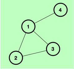
First let’s inductively construct the graph. We start with the empty graph [ ]. We insert node 3. Since it is the first node into the graph, it cannot reference any other nodes because they’re not in it yet. So our graph after inserting node three is [(3, [ ])]. Next, let’s insert node 2. It has an edge to node 3 which is already in the graph, so our graph after inserting node 2 looks like this: [(2, [3]), (3, [ ])]. Next we insert node 4 and get
[(4, [ ]), (2, [3]), (3, [ ])]. Finally we insert node 1 and get: [(1, [2,3,4]), (4, [ ]), (2, [3]), (3, [ ])].
Let’s do the same exercise but this time we insert the nodes in this order: 1, 4, 3, 2. We eventually
Node 2 gets in last so it is at the head of the sequence, ie the outermost context bound to the inductive graph. This is similar how cons and lists work.
get: [(2, [1, 3]), (3, [1]), (4, [1]), (1, [ ])].
Let’s call match on the first sequence of contexts, matching for node 2:
match 2 [(1, [2,3,4]), (4, [ ]), (2, [3]), (3, [ ])]
We get this result:
Just ((2,[1,3]),[(1,[3,4]),(4,[]),(3,[])])
Our DFS implementation is simple:
dfs :: [Node] -> Graph -> [Node]
dfs [] _ = []
dfs (v:vs) g = case m of
    Just (c, g') -> (fst c):(dfs ((snd c) ++ vs) g')
    Nothing -> dfs vs g
  where
    m = match v g
In the next part we will derive an inductive graph from a row matrix and then run DFS over that graph to check if the length of the returned visited nodes list is equal to the number of rows times number of ones, ie the magic square is connected.