
Imagine a 6 by 6 grid of squares, that can either be black or white.

It has to fulfill the following properties:
1. Each row and column needs to have 3 white and 3 black squares.
2. All black squares have to be orthogonally connected.

Prove that such a grid cannot exist.
- part 1: naive brute force exhaustive search
- part 2: smarter exhaustive search
- part 3: inductive graphs
- part 4: connected magic squares
- part 5: experiments
Note: in our digital representation black squares are ones and white squares are zeros.
This is part 2 of a series of posts about a puzzle I found on Mastodon and which I don’t yet know how to solve. In part 1 we decided to employ a brute force exhaustive search for solutions. There is a problem though, one very obvious if you look at the number of possible $n \times n$ matrices in $\mathbb{Z}_2$: $2^{n^2}$. The size of the exhaustive search literally grows exponentially. For a six by six matrix we have 68 billion possibilities. Unless you are very patient, doing the naive brute force won’t cut it.
We could try to speed up some of the operations. Because we are in $\mathbb{Z}_2$, we could replace div and mod by shiftR and .&.. The function binaryDigits' from part 1 becomes:
binaryDigits' :: Int -> [Int]
binaryDigits' 0 = [0]
binaryDigits' x = r : (binaryDigits' y)
   where
	  y = shiftR x 1
	  r = x .&. 1
We could also observe that in order to have $k$ ones in each row, the binary digit representation of our matrix possibilities must have ones in each row-length section of the digit sequence, so also in the most significant section.This means that our search interval is not [0..(2^(n * n) - 1)]] but rather [2^(n * (n -1))..(2^(n * n) - 1)]].
The function puzzleExamples from part 1 becomes:
puzzleExamples :: Int -> Int -> [[[Int]]]
puzzleExamples size numOnes = [m | Just m <- map (puzzleFilter size numOnes) [2^(size * (size -1))..(2^(size * size) - 1)]]
Unfortunately, this is still not good enough. If your problem space is an exponential function of the size $n$ as is the case here, then a thousand-fold increase in speed only buys you a couple of size increases of $n$. For our particular case (which is worse because it’s an exponential of the square of the size), those two improvements cannot handle the six by six case yet. We need a better approach.
Fortunately, it’s not that hard to come up with one: instead of blindly generating all matrices, why not start by at least generating rows that already have the right number of ones. If we also keep a tally of how many ones are in each column, we can eliminate even faster the matrices that violate the magic square property.
Let’s start with generating rows with a given number of ones. This sounds very much like generating all subsets of size $k$ from a set of size $n$, with the well-known Pascal-triangle recursion:
subsets :: Int -> [a] -> [[a]]
subsets 0 _ = [[]]
subsets _ [] = []
subsets k xs = (subsets k ys) ++ (map (x:) (subsets (k-1) ys))
  where
	x = head xs
	ys = tail xs
But here we’re not interested in the sets, but instead in the positional binary digit representation. We need to adjust the expressions a little. Let’s call the new function kones for $k$ ones:
kones :: Int -> Int-> [[Int]]
kones n 0 = [[0 | _ <- [1..n]]]
kones [] _ = []
kones n k = (map (1:) (kones (n-1) (k-1))) ++ (map (0:) (kones (n-1) k))
This gives us all the binary words of length $n$ with $k$ ones in them. These will form our rows in potential matrices. But we can do even better than this. Anticipating our column constraint needs, we could pass in a boolean list of positions where ones are allowed instead of passing in $n$:
kones :: [Bool] -> Int-> [[Int]]
kones cs 0 = [[0 | _ <- [1..n]]]
   where
	n = length cs
kones [] _ = []
kones (c:cs) k = if c then
	(map (1:) (kones cs (k-1))) ++ (map (0:) (kones cs k))
  else
	(map (0:) (kones cs k))
So the plan is this: we use kones to generate rows of a potential matrix while also keeping track of how many ones have accumulated in each column and forbidding ones in columns that have reached the limit.
We can set it up as described in chapter 15, pages 372-373 of:
Ideal for learning or reference, this book explains the five main principles of algorithm design and their implementation in Haskell.
Our State object is the matrix row list so far and the number of ones in each column so far, represented as a tuple:
type State = ([[Int]], [Int])
We move from State to new State with a Move which in our case will be a new row added to the matrix. We will do a depth-first search for solutions in this State space.
type Move = [Int]
Given a current state, we want to generate all the next moves that we want to consider:
moves :: Int -> State -> [Move]
moves k s = if ((length rows) == (Length csum)) then [] else kones cs k
  where
	(rows, csum) = s
	cs = map ((>) k) csum
If our state is already a square matrix, then no more moves are available. If not, we generate all the rows that put $k$ ones in columns that still have space.
Next we need a function that actually applies a given move to a state and produces a new state. This is simple in our case: the move row gets prepended to the current state matrix and the column sum vector gets updated by adding the new row to it so it reflects how many ones there are in each column in the new state.
move :: State -> Move -> State
move s m = (m:rows, map (\x -> (fst x) + (snd x)) (zip m cs))
  where
	(rows, cs) = s
And finally we need a function that judges a state and tells us if it is a valid solution, ie a magic square:
solved :: Int -> State -> Bool
solved k s = ((length rows) == (length cs)) && (allTrue (k ==) cs)
  where
    (rows, cs) = s
We don’t need to check the rows again since they have the right number of ones by construction (from the generated moves). We do need to check that all the columns have reached the number of ones limit, namely $k$ (a column could have fewer, but never more, again by construction).
We’re all set to do our DFS:
solutions :: Int -> State -> [State]
solutions k t = search k [t]

search :: Int -> [State] -> [State]
search _ [] = []
search k (t:ts) = if (solved k t) then t:(search k ts) else search k (succs k t ++ ts)

succs :: Int -> State -> [State]
succs k t = [move t m | m <- (moves k t)]
Our DFS is made up of three functions. The cover function solutions kicks things off with an initial state and calling search. search in turn checks if a state is a solution in which case it is prepended to the solutions. If it is not, then the successor states are generated with succs and prepended to whatever work is already pending, hence DFS.
So is it faster ? Yes, it is way faster. This returns instantly:
ghci> take 2 $ solutions 3 ([], [0, 0, 0, 0, 0, 0])
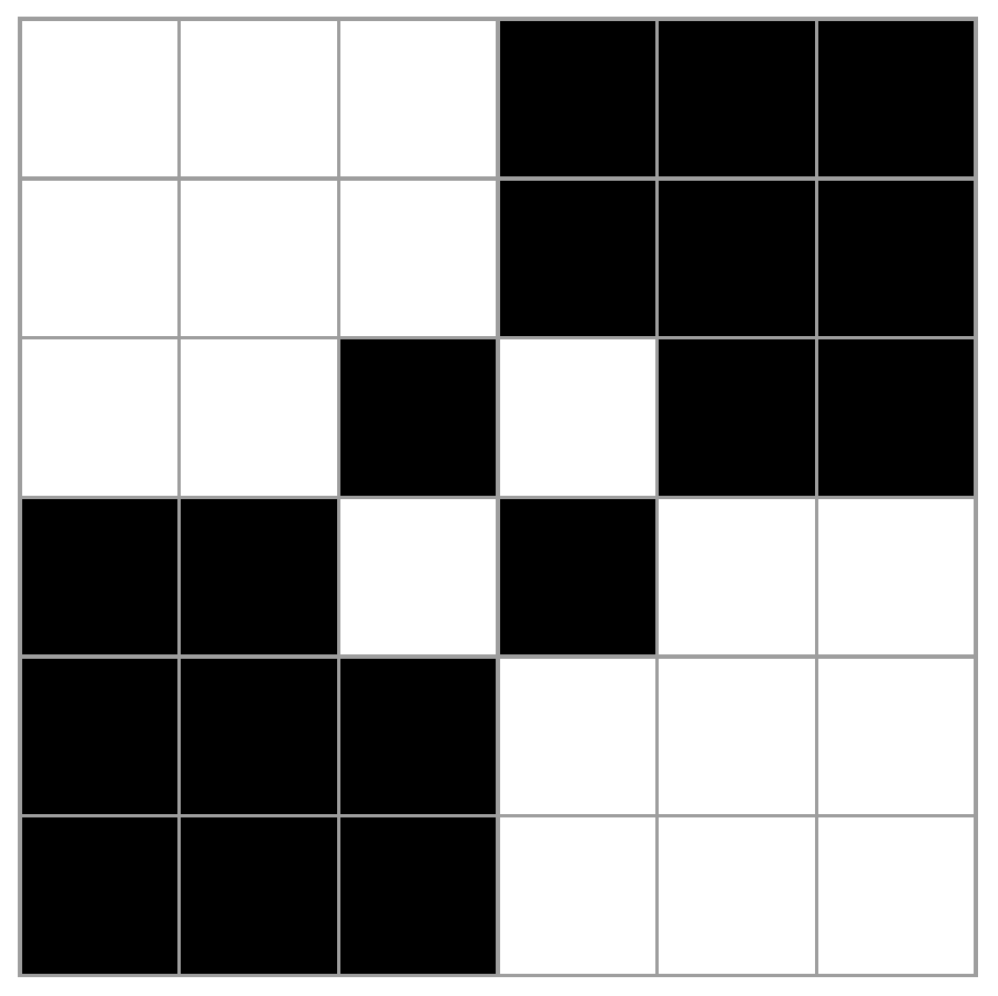
[([[0,0,0,1,1,1],[0,0,0,1,1,1],[0,0,0,1,1,1],[1,1,1,0,0,0],[1,1,1,0,0,0],[1,1,1,0,0,0]],[3,3,3,3,3,3]),([[0,0,0,1,1,1],[0,0,0,1,1,1],[0,0,1,0,1,1],[1,1,0,1,0,0],[1,1,1,0,0,0],[1,1,1,0,0,0]],[3,3,3,3,3,3])]
I said in part 1 that I didn’t want to do all this in Mathenatica because I prefer the simplicity and elegance of Haskell. But it still is nice to visually inspect the results, so I did write a small Mathematica function that given one of the above solutions as a string, does a matrix plot of it:
plotPuzzle[s_String] :=
 ArrayPlot[ToExpression[StringReplace[s, {"[" -> "{", "]" -> "}"}]],
  Mesh -> True]
We can copy-paste [[0,0,0,1,1,1],[0,0,0,1,1,1],[0,0,1,0,1,1],[1,1,0,1,0,0],[1,1,1,0,0,0],[1,1,1,0,0,0]] into it and get:
In the next installment, we’ll tackle connectedness and expand the solved function to eliminate matrices that are not connected.